Homework 9
Listing Count Data Files
main_folder<-'D:/Documents/UVM Classes/computational_bio/test_2025/OriginalData/NEON_count-landbird/'
print(main_folder)
## [1] "D:/Documents/UVM Classes/computational_bio/test_2025/OriginalData/NEON_count-landbird/"
subfolders <- list.dirs(main_folder, recursive = F)
print(subfolders)
##  [1] "D:/Documents/UVM Classes/computational_bio/test_2025/OriginalData/NEON_count-landbird/NEON.D01.BART.DP1.10003.001.2015-06.basic.20250129T000730Z.RELEASE-2025"
##  [2] "D:/Documents/UVM Classes/computational_bio/test_2025/OriginalData/NEON_count-landbird/NEON.D01.BART.DP1.10003.001.2016-06.basic.20250129T000730Z.RELEASE-2025"
##  [3] "D:/Documents/UVM Classes/computational_bio/test_2025/OriginalData/NEON_count-landbird/NEON.D01.BART.DP1.10003.001.2017-06.basic.20250129T000730Z.RELEASE-2025"
##  [4] "D:/Documents/UVM Classes/computational_bio/test_2025/OriginalData/NEON_count-landbird/NEON.D01.BART.DP1.10003.001.2018-06.basic.20250129T000730Z.RELEASE-2025"
##  [5] "D:/Documents/UVM Classes/computational_bio/test_2025/OriginalData/NEON_count-landbird/NEON.D01.BART.DP1.10003.001.2019-06.basic.20250129T000730Z.RELEASE-2025"
##  [6] "D:/Documents/UVM Classes/computational_bio/test_2025/OriginalData/NEON_count-landbird/NEON.D01.BART.DP1.10003.001.2020-06.basic.20250129T000730Z.RELEASE-2025"
##  [7] "D:/Documents/UVM Classes/computational_bio/test_2025/OriginalData/NEON_count-landbird/NEON.D01.BART.DP1.10003.001.2020-07.basic.20250129T000730Z.RELEASE-2025"
##  [8] "D:/Documents/UVM Classes/computational_bio/test_2025/OriginalData/NEON_count-landbird/NEON.D01.BART.DP1.10003.001.2021-06.basic.20250129T000730Z.RELEASE-2025"
##  [9] "D:/Documents/UVM Classes/computational_bio/test_2025/OriginalData/NEON_count-landbird/NEON.D01.BART.DP1.10003.001.2022-06.basic.20250129T000730Z.RELEASE-2025"
## [10] "D:/Documents/UVM Classes/computational_bio/test_2025/OriginalData/NEON_count-landbird/NEON.D01.BART.DP1.10003.001.2023-06.basic.20250129T000730Z.RELEASE-2025"
x <- c()

for (i in 1:10) {
  #setwd(subfolders[i])
  files<-list.files(path = subfolders[i], pattern = "countdata.*\\.csv$", full.names = TRUE)
  x <- c(x, files)
  return(x)
}

print(x)
## [1] "D:/Documents/UVM Classes/computational_bio/test_2025/OriginalData/NEON_count-landbird/NEON.D01.BART.DP1.10003.001.2015-06.basic.20250129T000730Z.RELEASE-2025/NEON.D01.BART.DP1.10003.001.brd_countdata.2015-06.basic.20241118T065914Z.csv"
library(upscaler)
library(dplyr)
library(stringr)
library(ggplot2)

source_batch(folder='Functions/')
## File "Functions//CalculateAbundance.R" sourced.
## File "Functions//CalculateRichness.R" sourced.
## File "Functions//CleanData.R" sourced.
## File "Functions//ExtractYear.R" sourced.
## File "Functions//FileLister.R" sourced.
## File "Functions//GenerateHistograms.R" sourced.
## File "Functions//RunRegression.R" sourced.
Reading in Data
# Read csv for each path in x
# Read all CSVs into a list of data frames
data_list <- lapply(x, read.csv)

library(dplyr)

combined_data <- do.call(rbind, lapply(x, function(path) {
  df <- read.csv(path)
  df %>%
    select(startDate, vernacularName, scientificName, taxonID)
}))

head(combined_data)
##           startDate               vernacularName       scientificName taxonID
## 1 2015-06-14T09:23Z               Red-eyed Vireo      Vireo olivaceus    REVI
## 2 2015-06-14T09:23Z Black-throated Green Warbler     Setophaga virens    BTNW
## 3 2015-06-14T09:23Z Black-throated Green Warbler     Setophaga virens    BTNW
## 4 2015-06-14T09:23Z      Black-and-white Warbler      Mniotilta varia    BAWW
## 5 2015-06-14T09:23Z       Black-capped Chickadee Poecile atricapillus    BCCH
## 6 2015-06-14T09:43Z      Black-and-white Warbler      Mniotilta varia    BAWW
Cleaning Data
#Cleaning Data

clean_data<-clean_data()

head(clean_data)
##   startDate               vernacularName       scientificName taxonID
## 1      2015               Red-eyed Vireo      Vireo olivaceus    REVI
## 2      2015 Black-throated Green Warbler     Setophaga virens    BTNW
## 3      2015 Black-throated Green Warbler     Setophaga virens    BTNW
## 4      2015      Black-and-white Warbler      Mniotilta varia    BAWW
## 5      2015       Black-capped Chickadee Poecile atricapillus    BCCH
## 6      2015      Black-and-white Warbler      Mniotilta varia    BAWW
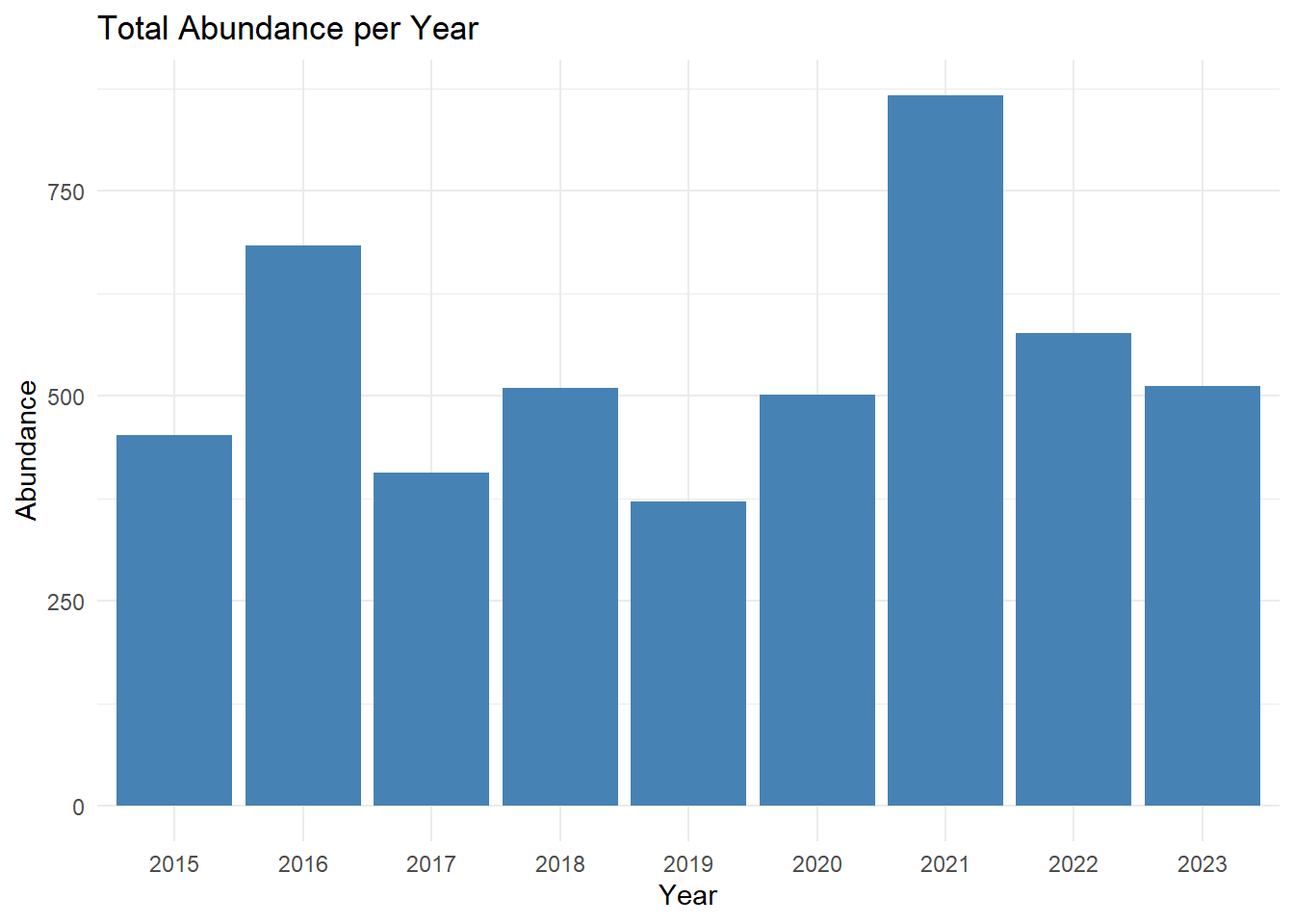
Calculating Abundance
#Function to calculate abundance

abundance<-calculate_abundance()
print(abundance)
## # A tibble: 9 × 2
##   startDate count
##   <chr>     <int>
## 1 2015        452
## 2 2016        684
## 3 2017        407
## 4 2018        510
## 5 2019        371
## 6 2020        501
## 7 2021        867
## 8 2022        577
## 9 2023        512
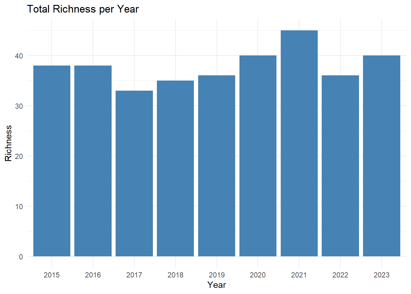
Calculating Richness
#Function to calculate species richness
richness<-calculate_richness()
print(richness)
## # A tibble: 9 × 2
##   startDate unique_species
##   <chr>              <int>
## 1 2015                  38
## 2 2016                  38
## 3 2017                  33
## 4 2018                  35
## 5 2019                  36
## 6 2020                  40
## 7 2021                  45
## 8 2022                  36
## 9 2023                  40
Linear Regression
#Simple Linear Regression
abundance_richness_df<-merge(richness,abundance,by='startDate')
colnames(abundance_richness_df) <- c("year", "richness",'abundance')
run_regression()
##
## Call:
## lm(formula = richness ~ abundance, data = abundance_richness_df)
##
## Coefficients:
## (Intercept)    abundance
##    28.63658      0.01706
Plotting Abundance and Richness
#generate abundance and richness plots

abundance_plot<-ggplot(data = abundance_richness_df, aes(x = factor(year), y = abundance)) +
    geom_col(fill = "steelblue") +
    labs(title = "Total Abundance per Year",
         x = "Year",
         y = "Abundance") +
    theme_minimal()
abundance_plot
richness_plot<-ggplot(data = abundance_richness_df, aes(x = factor(year), y = richness)) +
    geom_col(fill = "steelblue") +
    labs(title = "Total Richness per Year",
         x = "Year",
         y = "Richness") +
    theme_minimal()
richness_plot