Homework 8
Silas Decker
2025-03-19
Read in Fake Data Vector
library(ggplot2)
library(MASS)

# quick and dirty, a truncated normal distribution to work on the solution set

z <- rnorm(n=3000,mean=0.2)
z <- data.frame(1:3000,z)
names(z) <- list("ID","myVar")
z <- z[z$myVar>0,]
str(z)
## 'data.frame': 1724 obs. of 2 variables:
## $ ID : int 1 4 5 6 7 8 9 10 11 12 ...
## $ myVar: num 0.907 0.904 1.128 0.171 0.155 ...summary(z$myVar)## Min. 1st Qu. Median Mean 3rd Qu. Max.
## 0.001659 0.360947 0.763147 0.875324 1.260835 4.114252Plot Histogram of Data
p1 <- ggplot(data=z, aes(x=myVar, y=..density..)) +
  geom_histogram(color="grey60",fill="cornsilk",size=0.2)
print(p1)
## `stat_bin()` using `bins = 30`. Pick better value with `binwidth`.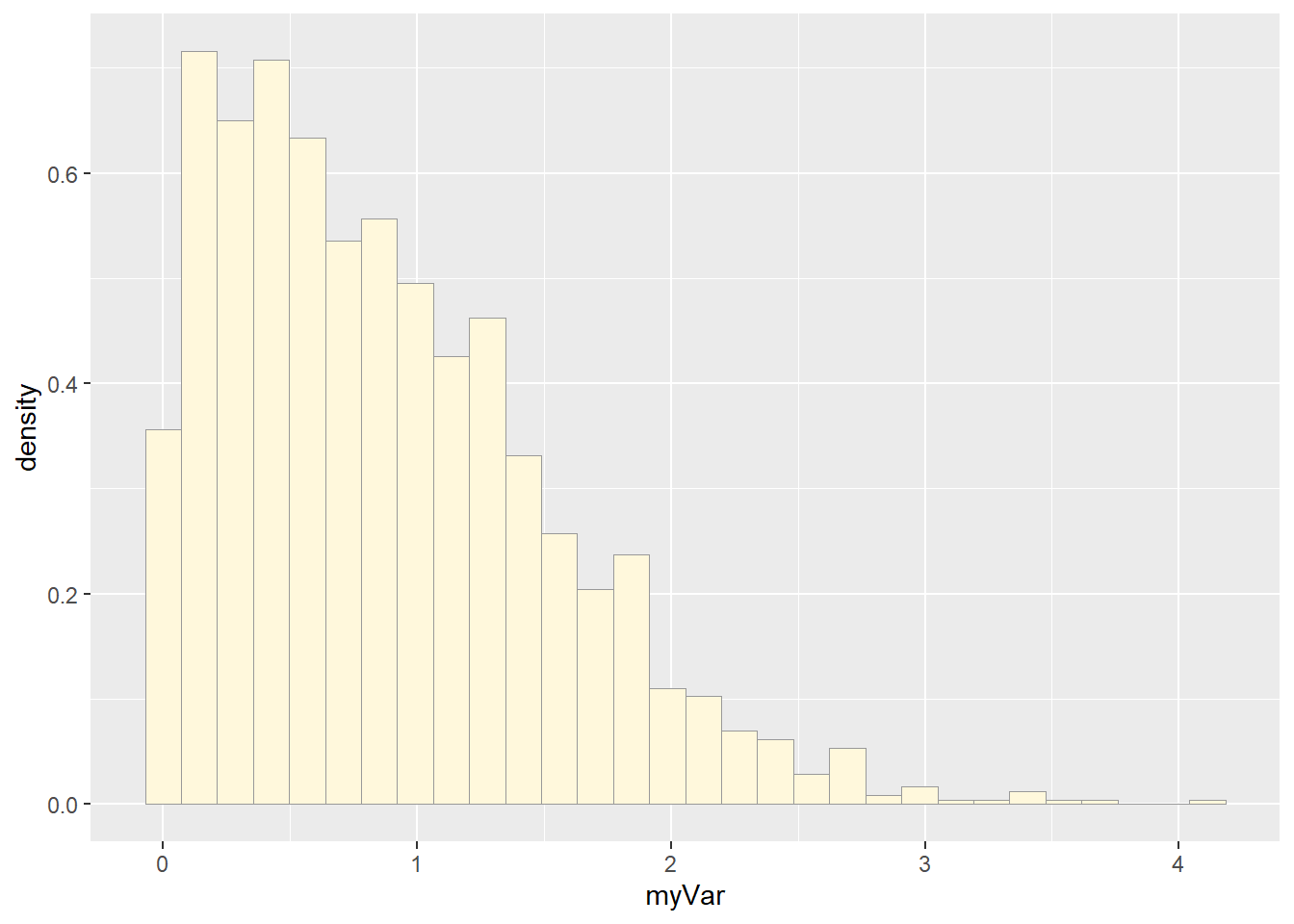
Empirical Density Curve
p1 <-  p1 +  geom_density(linetype="dotted",size=0.75)
print(p1)
## `stat_bin()` using `bins = 30`. Pick better value with `binwidth`.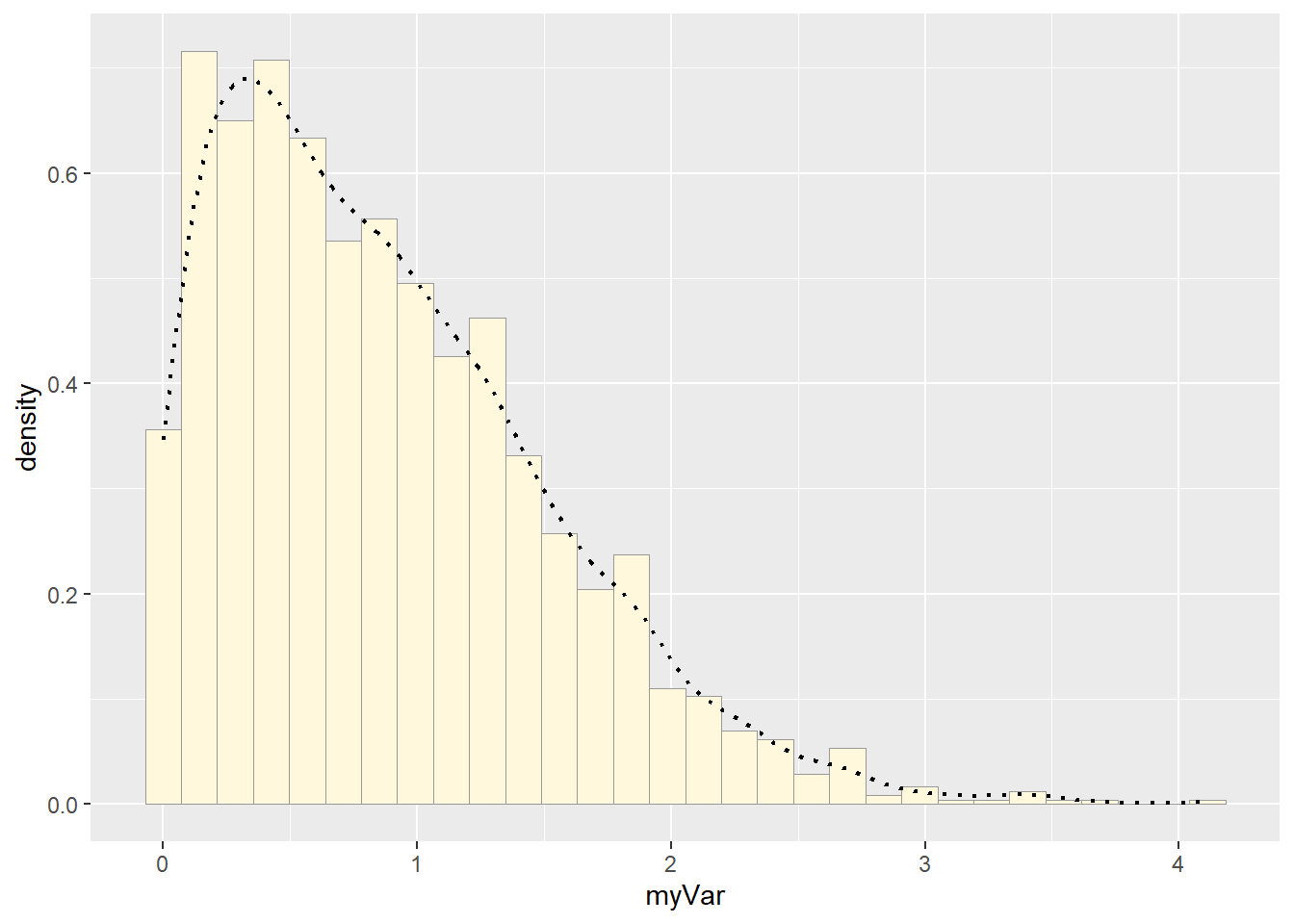
Maximum Likelihood Parameters for Normal
normPars <- fitdistr(z$myVar,"normal")
print(normPars)
## mean sd
## 0.87532439 0.64437664
## (0.01551927) (0.01097378)str(normPars)## List of 5
## $ estimate: Named num [1:2] 0.875 0.644
## ..- attr(*, "names")= chr [1:2] "mean" "sd"
## $ sd : Named num [1:2] 0.0155 0.011
## ..- attr(*, "names")= chr [1:2] "mean" "sd"
## $ vcov : num [1:2, 1:2] 0.000241 0 0 0.00012
## ..- attr(*, "dimnames")=List of 2
## .. ..$ : chr [1:2] "mean" "sd"
## .. ..$ : chr [1:2] "mean" "sd"
## $ n : int 1724
## $ loglik : num -1689
## - attr(*, "class")= chr "fitdistr"normPars$estimate["mean"] # note structure of getting a named attribute## mean
## 0.8753244Plot Normal PDF
meanML <- normPars$estimate["mean"]
sdML <- normPars$estimate["sd"]

xval <- seq(0,max(z$myVar),len=length(z$myVar))

 stat <- stat_function(aes(x = xval, y = ..y..), fun = dnorm, colour="red", n = length(z$myVar), args = list(mean = meanML, sd = sdML))
 p1 + stat
## `stat_bin()` using `bins = 30`. Pick better value with `binwidth`.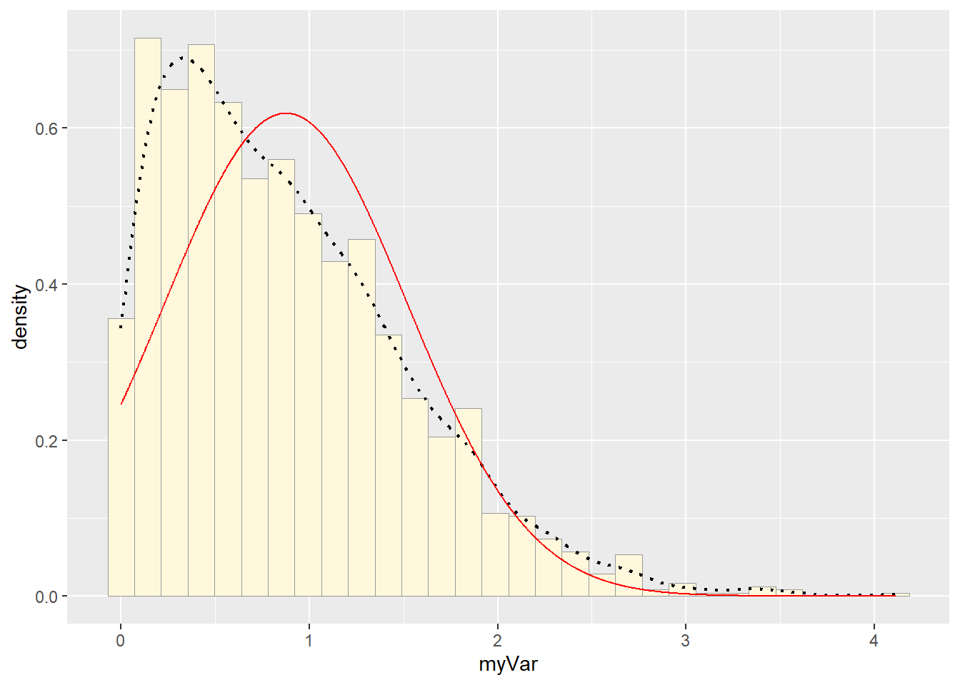 # Exponential PDF
expoPars <- fitdistr(z$myVar,"exponential")
rateML <- expoPars$estimate["rate"]

stat2 <- stat_function(aes(x = xval, y = ..y..), fun = dexp, colour="blue", n = length(z$myVar), args = list(rate=rateML))
 p1 + stat + stat2
## `stat_bin()` using `bins = 30`. Pick better value with `binwidth`.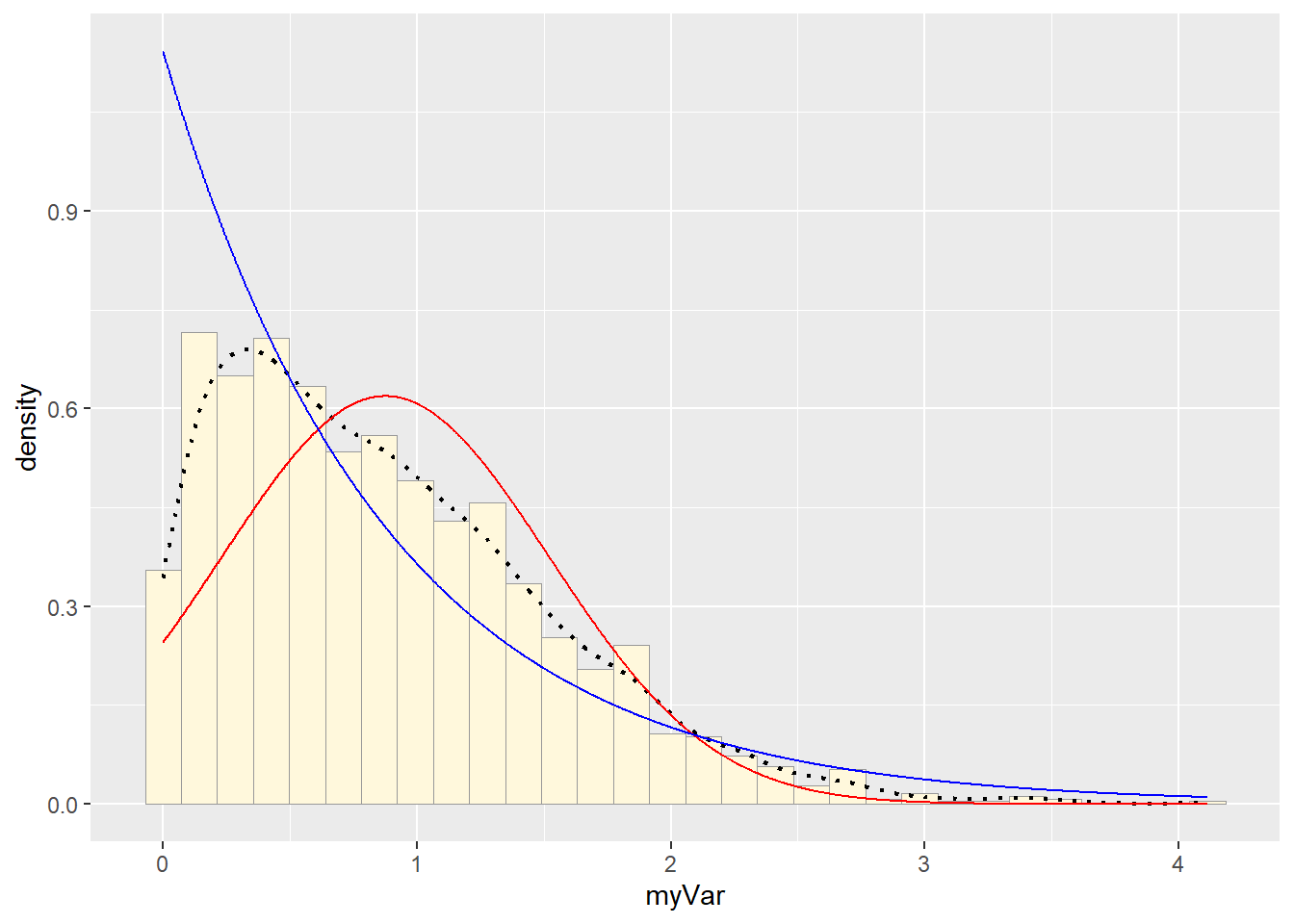 # Uniform PDF
stat3 <- stat_function(aes(x = xval, y = ..y..), fun = dunif, colour="darkgreen", n = length(z$myVar), args = list(min=min(z$myVar), max=max(z$myVar)))
 p1 + stat + stat2 + stat3
## `stat_bin()` using `bins = 30`. Pick better value with `binwidth`.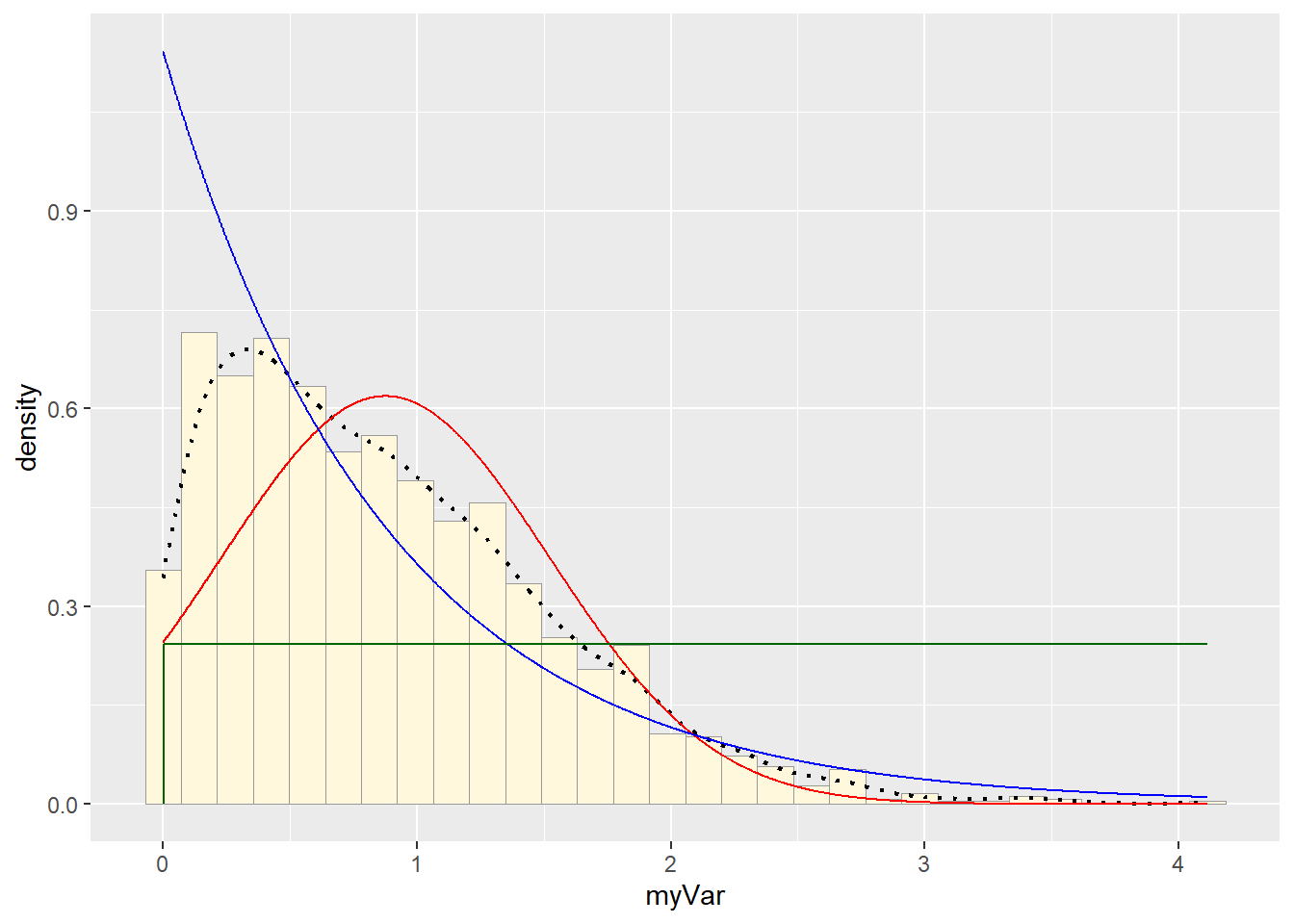 # Gamma PDF
gammaPars <- fitdistr(z$myVar,"gamma")## Warning in densfun(x, parm[1], parm[2], ...): NaNs produced
## Warning in densfun(x, parm[1], parm[2], ...): NaNs produced
## Warning in densfun(x, parm[1], parm[2], ...): NaNs produced
## Warning in densfun(x, parm[1], parm[2], ...): NaNs produced
## Warning in densfun(x, parm[1], parm[2], ...): NaNs produced
## Warning in densfun(x, parm[1], parm[2], ...): NaNs produced
## Warning in densfun(x, parm[1], parm[2], ...): NaNs producedshapeML <- gammaPars$estimate["shape"]
rateML <- gammaPars$estimate["rate"]
stat4 <- stat_function(aes(x = xval, y = ..y..), fun = dgamma, colour="brown", n = length(z$myVar), args = list(shape=shapeML, rate=rateML))
p1 + stat + stat2 + stat3 + stat4## `stat_bin()` using `bins = 30`. Pick better value with `binwidth`. # Beta PDF
pSpecial <- ggplot(data=z, aes(x=myVar/(max(myVar + 0.1)), y=..density..)) +
geom_histogram(color="grey60",fill="cornsilk",size=0.2) +
xlim(c(0,1)) +
geom_density(size=0.75,linetype="dotted")
betaPars <- fitdistr(x=z$myVar/max(z$myVar + 0.1),start=list(shape1=1,shape2=2),"beta")## Warning in densfun(x, parm[1], parm[2], ...): NaNs produced
## Warning in densfun(x, parm[1], parm[2], ...): NaNs produced
## Warning in densfun(x, parm[1], parm[2], ...): NaNs produced
## Warning in densfun(x, parm[1], parm[2], ...): NaNs produced
## Warning in densfun(x, parm[1], parm[2], ...): NaNs producedshape1ML <- betaPars$estimate["shape1"]
shape2ML <- betaPars$estimate["shape2"]
statSpecial <- stat_function(aes(x = xval, y = ..y..), fun = dbeta, colour="orchid", n = length(z$myVar), args = list(shape1=shape1ML,shape2=shape2ML))
pSpecial + statSpecial## `stat_bin()` using `bins = 30`. Pick better value with `binwidth`.## Warning: Removed 2 rows containing missing values or values outside the scale range
## (`geom_bar()`).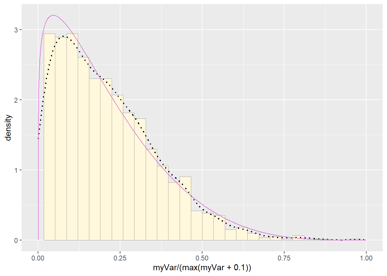
Real Data Time
library(tidyverse)
pfas<-read.csv('pfas.csv')
head(pfas)## gm_chemical_name gm_result_modifier gm_result
## 1 N-Methyl perfluorooctane sulfonamidoacetic acid (NMeFOSAA) < 1.7
## 2 Perfluorononanoic acid (PFNA) < 1.7
## 3 Perfluorododecanoic acid (PFDoDA) < 1.7
## 4 Perfluorotridecanoic acid (PFTrDA) < 1.7
## 5 Perfluorotetradecanoic acid (PFTeDA) < 1.7
## 6 Perfluoroundecanoic acid (PFUnDA) < 1.7pfas_num<-pfas %>%
select(gm_chemical_name, gm_result)
pfas_num_clean<-pfas_num[complete.cases(pfas_num),]
#add log column for the results
pfas_num_clean$log_gm_result <- log10(pfas_num_clean$gm_result)
pfas_num_clean <- pfas_num_clean[pfas_num_clean$log_gm_result > 0 & pfas_num_clean$log_gm_result < 1, ]
pfas_num_clean <- pfas_num_clean[is.finite(pfas_num_clean$log_gm_result), ]
# Clean data
#sum(is.na(pfas_num_clean$log_gm_result))Plot Histogram of Data
# using log scale to get better view of data
p1 <- ggplot(data=pfas_num_clean, aes(x=log_gm_result, y=..density..)) +
geom_histogram(binwidth=.10,color="grey60",fill="cornsilk",size=.2)
#scale_x_log10()
print(p1)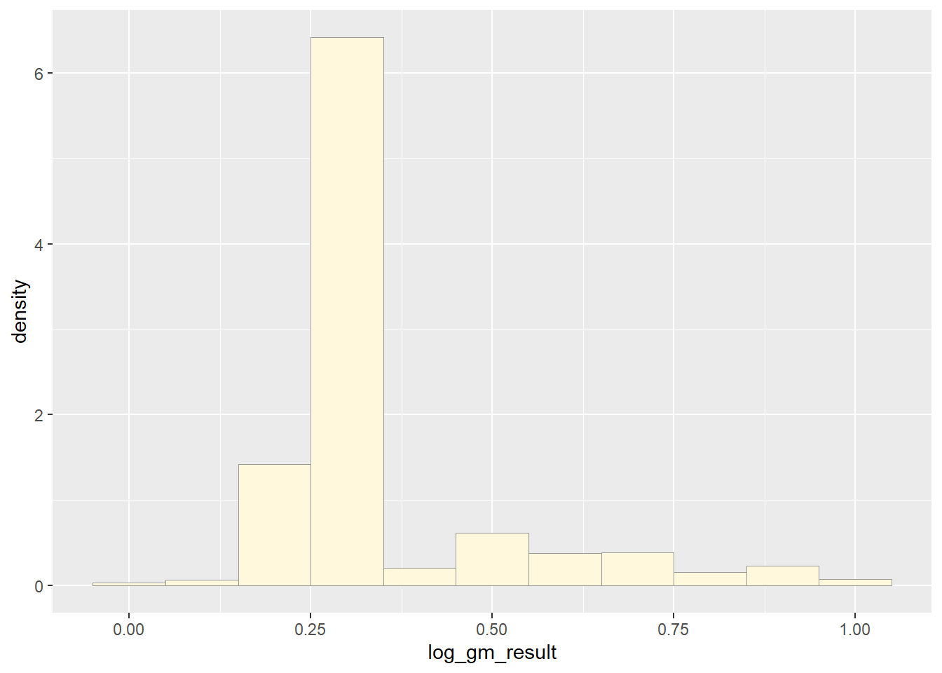
#str(z)
#str(pfas_num_clean)
#str(pfas_num_clean$gm_result)
#summary(pfas_num_clean$gm_result)Empirical Density Curve
p1 <- p1 + geom_density(linetype="dotted",size=0.75)
print(p1)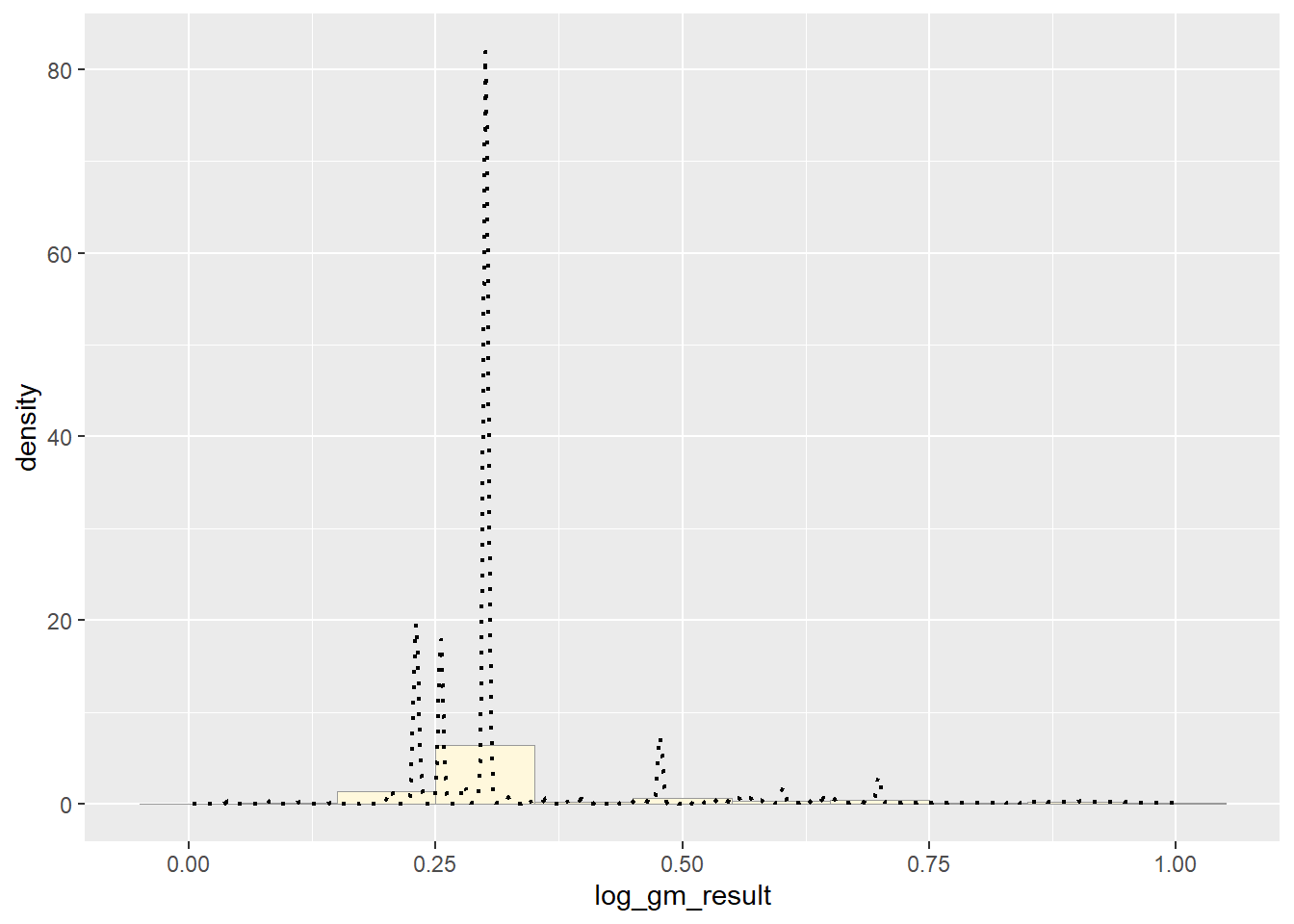
Maximum Likelihood Parameters for Normal
library(MASS)
pfas_num_clean <- pfas_num_clean[is.finite(pfas_num_clean$log_gm_result), ]
normPars <- fitdistr(pfas_num_clean$log_gm_result,"normal")
print(normPars)## mean sd
## 0.3504861641 0.1632875055
## (0.0002200754) (0.0001556168)str(normPars)## List of 5
## $ estimate: Named num [1:2] 0.35 0.163
## ..- attr(*, "names")= chr [1:2] "mean" "sd"
## $ sd : Named num [1:2] 0.00022 0.000156
## ..- attr(*, "names")= chr [1:2] "mean" "sd"
## $ vcov : num [1:2, 1:2] 4.84e-08 0.00 0.00 2.42e-08
## ..- attr(*, "dimnames")=List of 2
## .. ..$ : chr [1:2] "mean" "sd"
## .. ..$ : chr [1:2] "mean" "sd"
## $ n : int 550507
## $ loglik : num 216517
## - attr(*, "class")= chr "fitdistr"normPars$estimate["mean"] # note structure of getting a named attribute## mean
## 0.3504862Plot Normal PDF
meanML <- normPars$estimate["mean"]
sdML <- normPars$estimate["sd"]
xval <- seq(0,max(pfas_num_clean$log_gm_result),len=length(pfas_num_clean$log_gm_result))
stat <- stat_function(aes(x = xval, y = ..y..), fun = dnorm, colour="red", n = length(pfas_num_clean$log_gm_result), args = list(mean = meanML, sd = sdML))
p1 + stat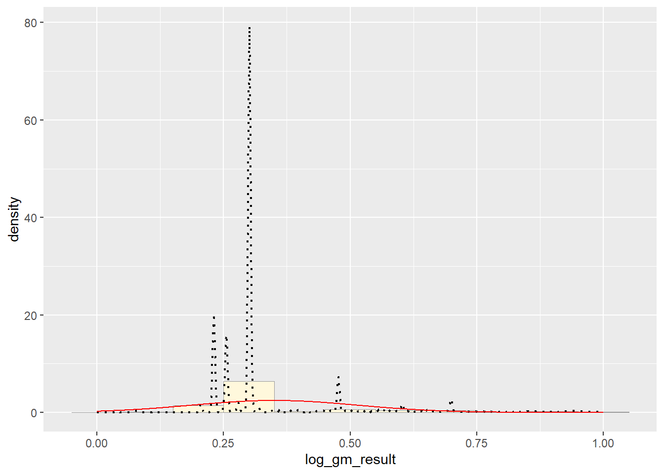 # Exponential PDF
expoPars <- fitdistr(pfas_num_clean$log_gm_result,"exponential")
rateML <- expoPars$estimate["rate"]
stat2 <- stat_function(aes(x = xval, y = ..y..), fun = dexp, colour="blue", n = length(pfas_num_clean$log_gm_result), args = list(rate=rateML))
p1 + stat + stat2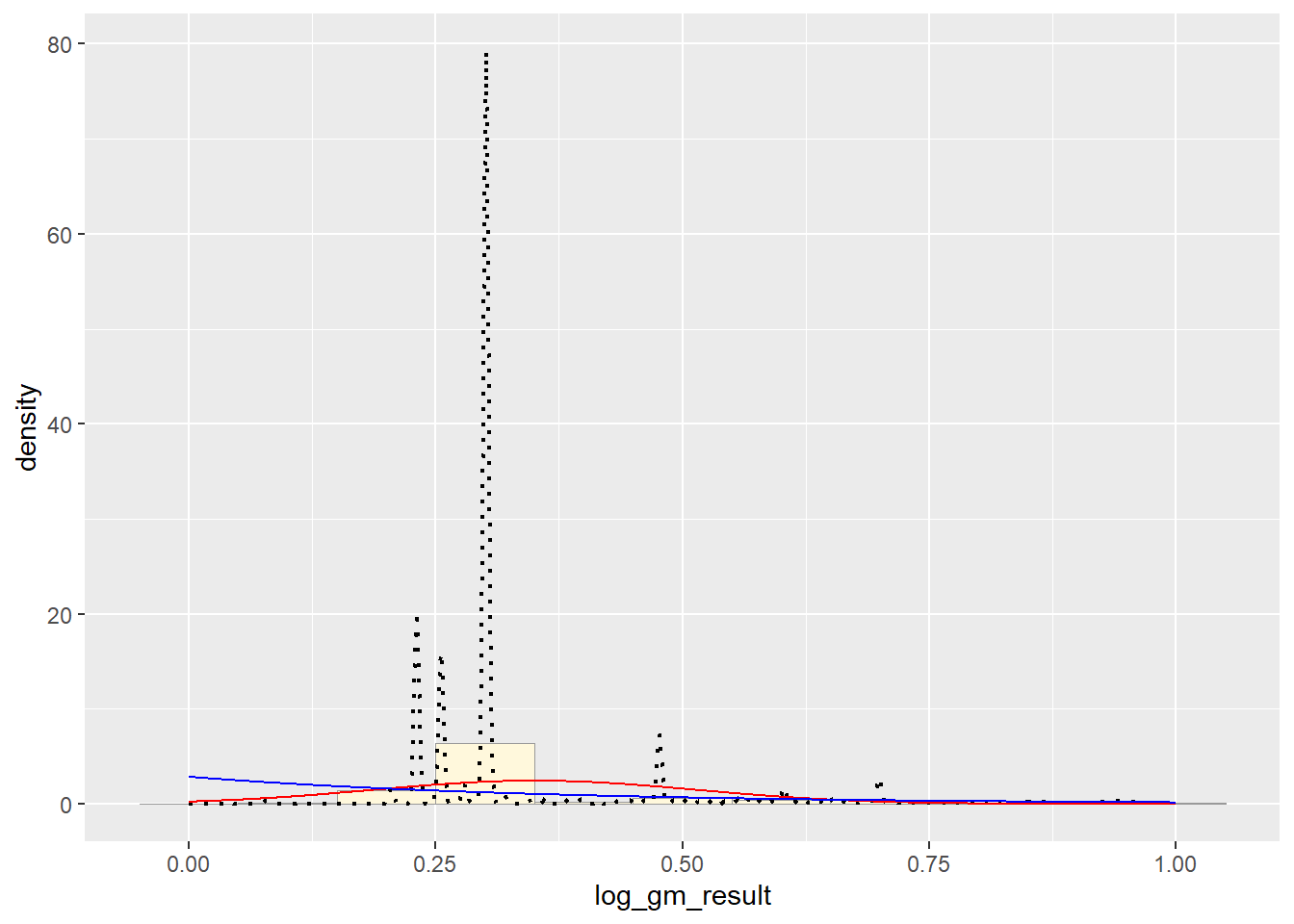 # Uniform PDF
stat3 <- stat_function(aes(x = xval, y = ..y..), fun = dunif, colour="darkgreen", n = length(pfas_num_clean$log_gm_result), args = list(min=min(pfas_num_clean$log_gm_result), max=max(pfas_num_clean$log_gm_result)))
p1 + stat + stat2 + stat3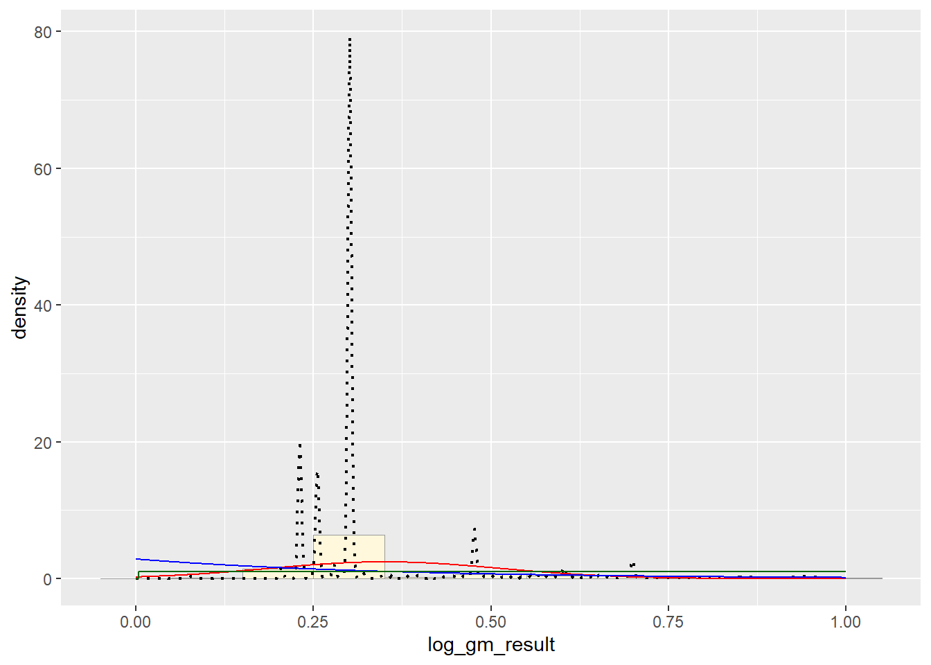 # Gamma PDF
gammaPars <- fitdistr(pfas_num_clean$log_gm_result,"gamma")## Warning in densfun(x, parm[1], parm[2], ...): NaNs producedshapeML <- gammaPars$estimate["shape"]
rateML <- gammaPars$estimate["rate"]
stat4 <- stat_function(aes(x = xval, y = ..y..), fun = dgamma, colour="brown", n = length(pfas_num_clean$log_gm_result), args = list(shape=shapeML, rate=rateML))
p1 + stat + stat2 + stat3 + stat4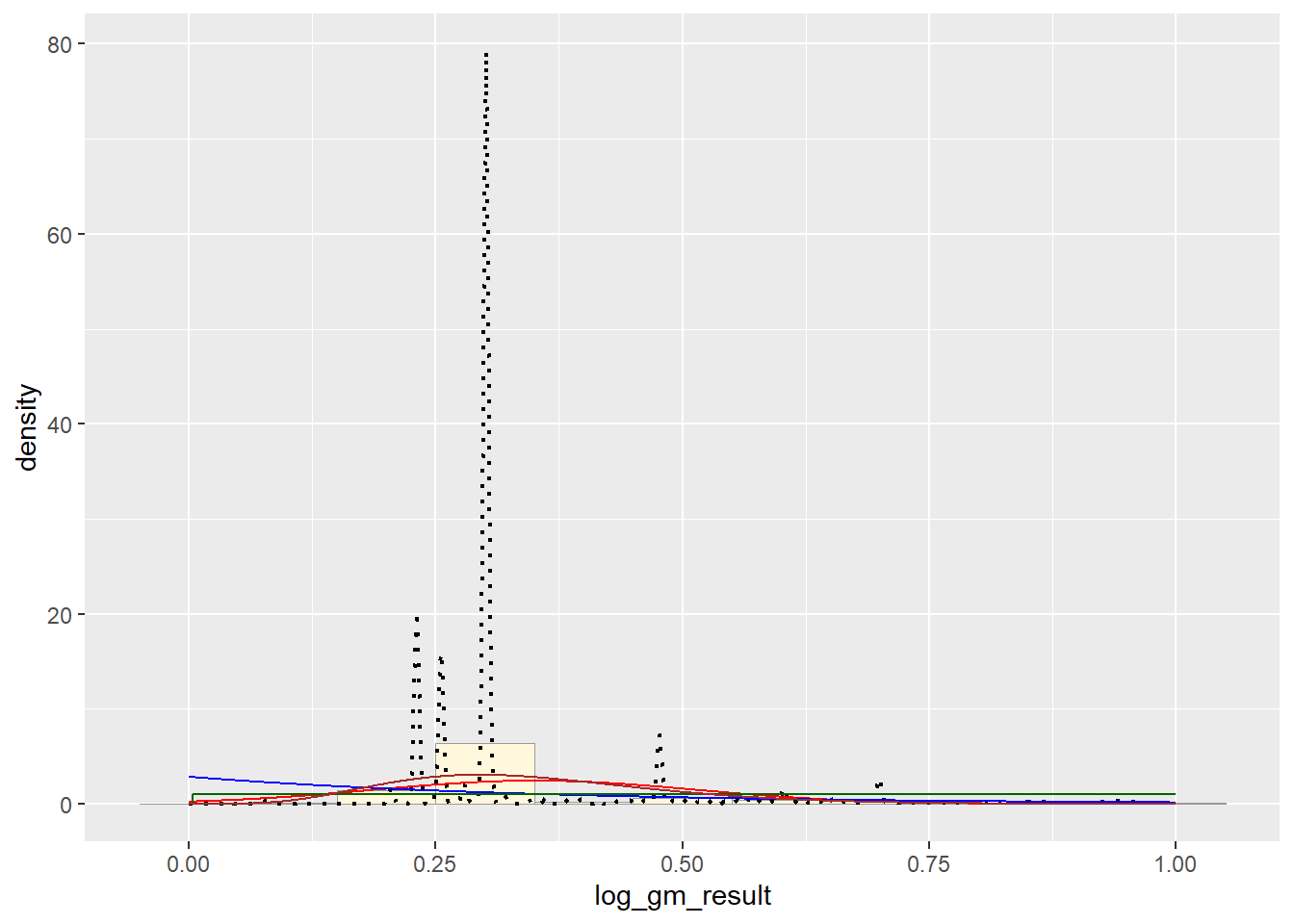 # Beta PDF
pSpecial <- ggplot(data=pfas_num_clean, aes(x=log_gm_result/(max(log_gm_result + 0.1)), y=..density..)) +
geom_histogram(color="grey60",fill="cornsilk",size=0.2) +
xlim(c(0,1)) +
geom_density(size=0.75,linetype="dotted")
betaPars <- fitdistr(x=pfas_num_clean$log_gm_result/max(z$myVar + 0.1),start=list(shape1=1,shape2=2),"beta")## Warning in densfun(x, parm[1], parm[2], ...): NaNs produced
## Warning in densfun(x, parm[1], parm[2], ...): NaNs produced
## Warning in densfun(x, parm[1], parm[2], ...): NaNs produced
## Warning in densfun(x, parm[1], parm[2], ...): NaNs produced
## Warning in densfun(x, parm[1], parm[2], ...): NaNs produced
## Warning in densfun(x, parm[1], parm[2], ...): NaNs produced
## Warning in densfun(x, parm[1], parm[2], ...): NaNs produced
## Warning in densfun(x, parm[1], parm[2], ...): NaNs produced
## Warning in densfun(x, parm[1], parm[2], ...): NaNs produced
## Warning in densfun(x, parm[1], parm[2], ...): NaNs produced
## Warning in densfun(x, parm[1], parm[2], ...): NaNs produced
## Warning in densfun(x, parm[1], parm[2], ...): NaNs produced
## Warning in densfun(x, parm[1], parm[2], ...): NaNs produced
## Warning in densfun(x, parm[1], parm[2], ...): NaNs produced
## Warning in densfun(x, parm[1], parm[2], ...): NaNs produced
## Warning in densfun(x, parm[1], parm[2], ...): NaNs produced
## Warning in densfun(x, parm[1], parm[2], ...): NaNs produced
## Warning in densfun(x, parm[1], parm[2], ...): NaNs produced
## Warning in densfun(x, parm[1], parm[2], ...): NaNs produced
## Warning in densfun(x, parm[1], parm[2], ...): NaNs producedshape1ML <- betaPars$estimate["shape1"]
shape2ML <- betaPars$estimate["shape2"]
statSpecial <- stat_function(aes(x = xval, y = ..y..), fun = dbeta, colour="orchid", n = length(pfas_num_clean$log_gm_result), args = list(shape1=shape1ML,shape2=shape2ML))
pSpecial + statSpecial## `stat_bin()` using `bins = 30`. Pick better value with `binwidth`.## Warning: Removed 2 rows containing missing values or values outside the scale range
## (`geom_bar()`).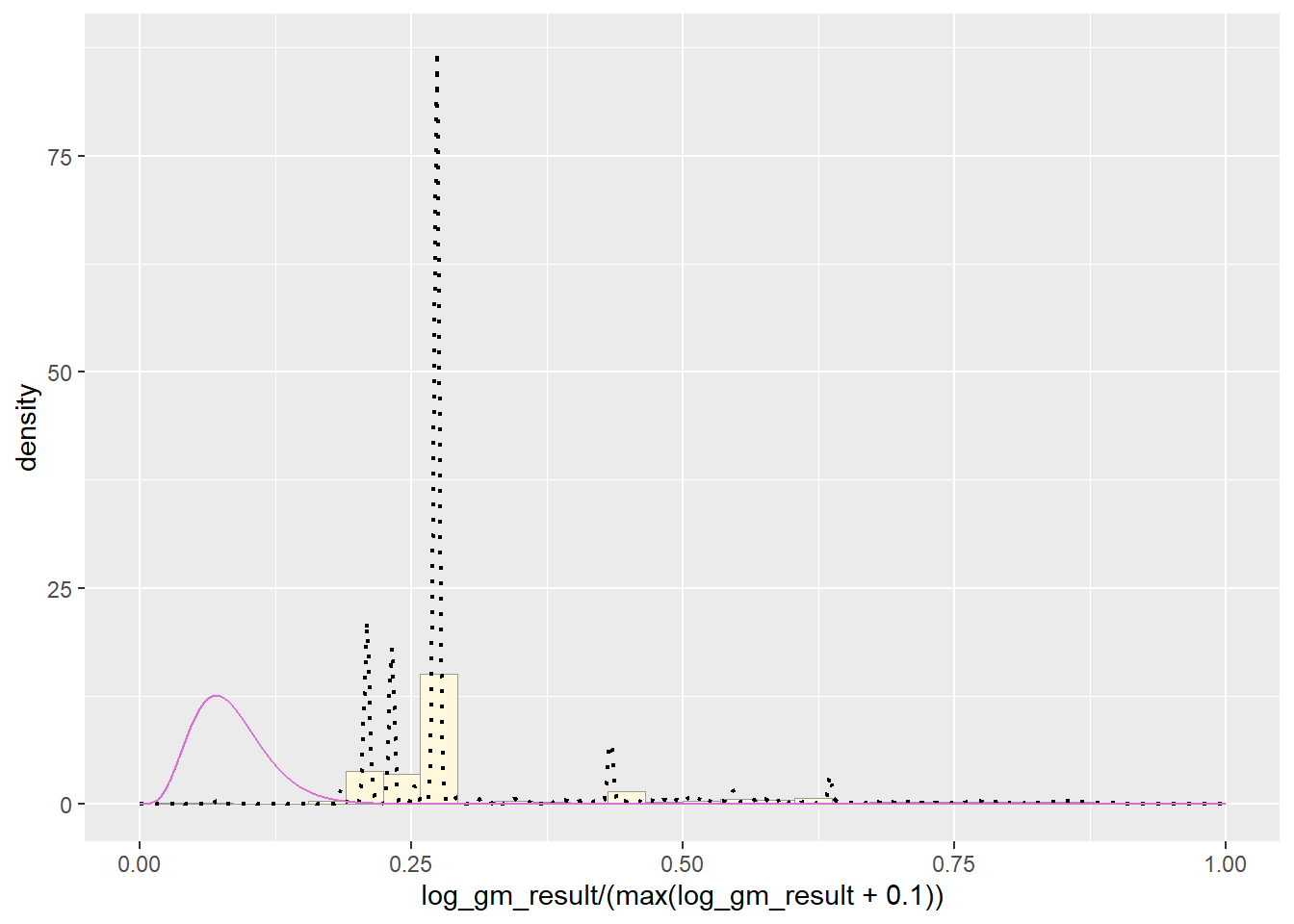
Write up/discussion
Upon completing the probability functions, my data is clearly a little whack. The original data had a massive range of values from 0 to hundreds of thousands. In order to improve the distribution I took the log value of the values of pfas and then truncated it between 0 and 100. This provided a better histogram, as the raw data was just one bar, but it still was not a pretty shape.
It appears that the best fit is the Normal PDF, in that it encompasses the shape of the data better than the other functions. However, I still believe that these functions did not do a good job overall with fitting the data. Each curve seems to be a somewhat different trajectory than the data’s histogram follows. I am not positive as to what contributed to this, though I reckon it still has to do with the high degree of variance seen in my data set.